| Average SPSS minutes | Average # obscenities |
|---|---|
| 240 | 3 |
| 310 | 6 |
| 230 | 4 |
| 220 | 3 |
3 Correlation coefficients and working with normal distributions
3.1 Learning goals
3.1.1 Conceptual
- Calculate and interpret pearson’s \(r\) by hand
- Z-transform datapoints and interpret the result
3.1.2 SPSS
- Compute pearson’s \(r\)
3.2 Pearson’s \(r\) correlation coefficient
Pearson’s \(r\) is given by:
\[
r_{xy} = \frac{\sum_{i=1}^{n}{(x_i - \bar{x})(y_i - \bar{y})}}{{\sqrt{\sum_{i=1}^{n}{(x_i - \bar{x})^2}}}{\sqrt{\sum_{i=1}^{n}{(y_i - \bar{y})^2}}}}
\]
Where:
- \(x_i\) = i’th score on variable \(x\)
- \(y_i\) = i’th score on variable \(y\)
- \(\bar{x}\) = mean of variable \(x\)
- \(\bar{y}\) = mean of variable \(y\)
- \(\sum_{i=1}^{n}\) = sum scores from index (element) 1 to \(n\)
- \(n\) = sample size
Let’s now imagine that we develop the following Research Question:Does the average daily time (in minutes) spent using SPSS correlate with the average number of obscenities used per day? We collect some data, which looks like this:
With the following steps, we can unpack the formula and derive the correlation coefficient:
| $$x_{minutes}$$ | $$y_{words}$$ | $$x-\bar{x}$$ | $$y-\bar{y}$$ | $$(x-\bar{x}).(y-\bar{y})$$ | $$(x-\bar{x})^2$$ | $$(y-\bar{y})^2$$ |
|---|---|---|---|---|---|---|
| 240 | 3 | -10 | -1 | 10 | 100 | 1 |
| 310 | 6 | 60 | 2 | 120 | 3600 | 4 |
| 230 | 4 | -20 | 0 | 0 | 400 | 0 |
| 220 | 3 | -30 | -1 | 30 | 900 | 1 |
- \(\bar{x} = 250\)
- \(\bar{y}= 4\)
- \(\sum_{i=1}^{n}{(x_i - \bar{x})(y_i - \bar{y})}=160\)
- \(\sum_{i=1}^{n}{(x_i - \bar{x})^2} = 5000\)
- \(\sum_{i=1}^{n}{(y_i - \bar{y})^2} = 6\)
\[
r_{xy} = \frac{160}{\sqrt{5000}*\sqrt{6}} = \frac{160}{173.21} = .92
\]
We will use the following rules-of-thumb for interpreting absolute values of \(r\):
- \(r \le .3\) = small
- \(.3 < r \le .6\) = moderate
- \(.6 < r \le .8\) = strong
- \(.8 < r \le 1\) = very strong
3.3 Z-transformations
Imagine we know that income per week (in euro) is normally distributed in the population of Dutch university students who graduated in the last year, such that the mean (\(\mu\)) income is 1,500 EUR, with an SD (\(\sigma\)) of 100. We might wonder: what proportion of the population of new Dutch graduates would have a weekly income of greater than 1,700 EUR?
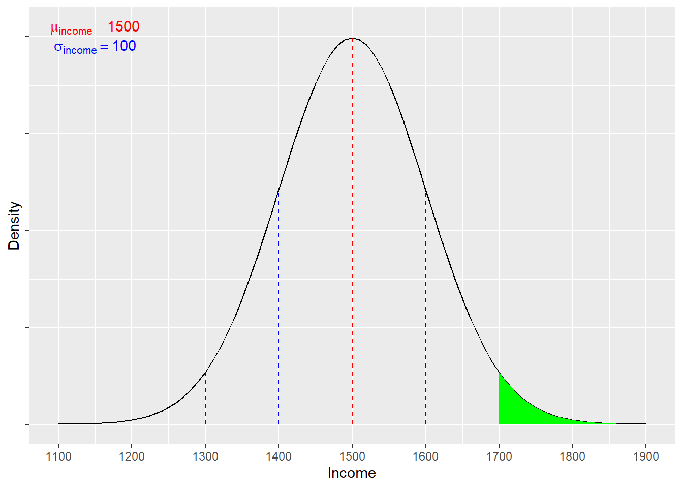
We can see the area of interest in the distribution above, in Figure 3.1. To calculate the proportion, we first need to convert the target value into a z-score, which transforms the value into standard deviation units. In this case:
\[ z = \frac{x-\mu}{\sigma} = \frac{1700-1500}{100} = 2 \]
To work out the probability associated with a z-score of 2, we can consult the normal distribution tables in the Argyrous textbook (pp. 541 - 542), looking for the area under the curve beyond one point. This allows us to answer our question: there is a 2.28% chance of randomly selecting an individual with an income above 1,700 EUR per week from the population of new Dutch graduates
3.4 Scatterplots and \(r\) with the WDI data (SPSS)
Let’s again load in the World Data Indicators (WDI) dataset (World_Data.sav), and revisit our scatterplot from the previous class (see Figure 2.1).
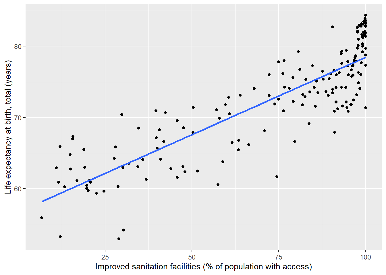
We see a noisy, yet positive relationship between a country’s percentage access to improved sanitation and its life expectancy at birth. The points do not cling to the linear fit line, but are scattered around it.
To give us some more formal information about the relationship strength, we can calculate pearson’s \(r\) in SPSS which reveals that the correlation between the variables is 0.86. Following our rules-of-thumb above, we could diagnose this as a very strong, positive relationship between the two variables.
3.5 SPSS explainer video (World Data)
- Scatterplots
- Pearson’s \(r\)
Note that I refer to a strong correlation in the video, when this should be very strong, following our rules of thumb.↩︎