Sex |
|||
|---|---|---|---|
| Signed? | Male | Female | Total |
| Yes | 7 | 20 | 27 |
| No | 40 | 25 | 65 |
| Total | 47 | 45 | 92 |
6 The \(\chi^2\) test of independence, the independent-samples t-test, and the paired-samples t-test
6.1 Learning goals
6.1.1 Conceptual
- Calculate the \(\chi^2\) statistic by hand and determine its significance
6.1.2 SPSS
Run and interpret the:
- \(\chi^2\) test of independence
- independent-samples t-test
- paired-samples t-test
6.2 \(\chi^2\) test of independence by hand
This test is appropriate when we wish to examine the relationship between two variables which are measured either at the nominal or ordinal. For example, we might have a research question such as: Is there a relationship between sex and having signed a petition in the last 12 months among the UvA student population? If we operationalize ‘sex’ as ‘female/male’ and ‘petition signed in the last 12 months’ as ‘yes/no’, then we have two nominal (binary) variables. As we will one more use crosstabulations to visualize the relationship between these two variables, we will nominate ‘sex’ as our independent variable, as, were there any causal relationship between these variables, it would surely originate with ‘sex’ and not the other way around.
Having defined our variables, we can specify hypotheses for our test:
- \(H_0\) = In the population of UvA students, there is no relationship between sex and having signed a petition in the last 12 months
- \(H_1\) = In the population of UvA Students, there IS a relationship between sex and having signed a petition in the last 12 months
Now, let’s make a crosstabulation of the data:
As we do not have equal numbers of female and male participants, we can compute column percentages as previously:
Sex |
|||
|---|---|---|---|
| Signed? | Male | Female | Total |
| Yes | 14.89 | 44.44 | 29.35 |
| No | 85.11 | 55.56 | 70.65 |
| Total | 100.00 | 100.00 | 100.00 |
With this descriptive tabulation, we can see that female students appear to have signed petitions more often in the last 12 months than male students. So, we have a suggestion that the two variables are related, but, in order to make inferences about the population, we need to compute the \(\chi^2\) statistic from the counts. Put simply, this statistic tells us how much the observed frequencies in each cell deviate from the pattern expected under the null hypothesis (i.e., that there is no relationship between the variables.) If you look at the distribution of counts for ‘Yes’ and ‘No’ in the ‘Total’ column, you can see the expected pattern if the data were to be collapsed across ‘Sex’. These totals allow us to calculate the expected frequencies of petition signing for both females and males, which we can compare to the observed frequencies as part of our calculation of the \(\chi^2\) test statistic:
\[ \chi^2 = \sum \frac{(f_o - f_e)^2}{f_e} \tag{6.1}\]
Where:
- \(f_o\) = observed frequencies
- \(f_e\) = expected frequencies
- Frequencies we expect to find in each cell if IV and DV are unrelated (i.e., under \(H_0\))
Sex |
|||
|---|---|---|---|
| Signed? | Male | Female | Total |
| Yes | 7 | 20 | 27 (29.35%) |
| No | 40 | 25 | 65 (70.65%) |
| Total | 47 | 45 | 92 (100%) |
Given our totals, we can calculate the expected frequencies as follows:
- female/yes: \(f_e = \frac{29.35}{100} \times 45 = 13.21\)
- female/no: \(f_e = \frac{70.65}{100} \times 45 = 31.79\)
- male/yes: \(f_e = \frac{29.35}{100} \times 47 = 13.79\)
- male/no: \(f_e = \frac{70.65}{100} \times 47 = 33.21\)
Recalling the equation, we can calculate the statistic step-by-step:
| $$f_o$$ | $$f_e$$ | $$(f_o - f_e)^2$$ | $$(f_o - f_e)^2/f_e$$ |
|---|---|---|---|
| 7 | 13.79 | 46.1 | 3.34 |
| 20 | 13.21 | 46.1 | 3.49 |
| 40 | 33.21 | 46.1 | 1.39 |
| 25 | 31.79 | 46.1 | 1.45 |
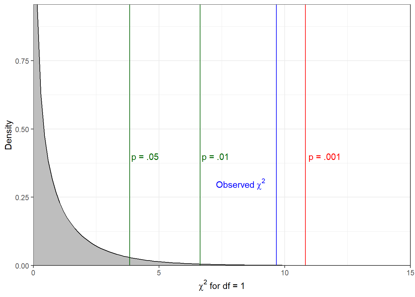
Summing the squared differences between the observed and expected frequencies in the rightmost column gives us a \(\chi^2\) score of 9.67. In order to determine the significance of the statistic, we need to consult the statistical table A4 on page xx of the Argyrous book. The degrees of freedom value for the test is calculated by subtracting 1 from the number of rows and columns, and multiplying the result. As we have two rows and two columns, this test has 1 degree of freedom, and we can therefore find the relevant critical \(\chi^2\) statistics in the first row of the table. We begin by comparing our value to the critical value associated with the .05 level, which our observed value exceeds. We repeat this process with the thresholds in the table until we find a critical value greater than our observed value, in this case the value associated with the .001 significance level. The significance level we report, then, is the value to the left of this (i.e., the lowest significance value whose critical value is exceeded by our observed value). The figure below shows a \(\chi^2\) distribution with 1 degree of freedom, with notations at the critical values for the significance levels referenced in the textbook, and at the observed statistic.
6.2.1 Reporting results
- A Chi-Square test of independence showed a significant relationship between gender and having signed a petition in the last month, \(\chi^2\)(1, N=92) = 9.67, p< 0.01.
- (We reject \(H_0\) with p < 0.01).
- (We reject \(H_0\) with p < 0.01).
- Plainly: in the population, there appears to be a relationship between gender and whether or not people have signed a petition in last 12 months: women are more likely to have signed a petition.
6.3 The independent-samples t-test
The independent-samples t-test is useful when we want to compare two mutually exclusive groups’ scores on a single dependent variable. For example, we may wish to compare reduction on depression inventory scores among patients who were randomized to receive either a new drug or the best current drug. For this test, we specify hypotheses about population mean differences among the groups, as follows:
- \(H_0: \mu_{new} = \mu_{current}\)
- ‘In the population of depression patients, there is no difference in the average effects of the new drug treatment and the current drug treatment.’
- \(H_{1a}: \mu_{new} \neq \mu_{current}\)
- ‘In the population of depression patients, there is a difference in the average effects of the new drug treatment and the current drug treatment.’ (non-directional)
- \(H_{1b}: \mu_{new} > \mu_{current}\)
- ‘In the population of depression patients, there is a greater average effect of the new drug treatment as compared to the current drug treatment.’ (directional)
6.4 The paired-samples t-test
The paired-samples t-test is of use in the following scenarios:
- Where we collect two measurements of a dependent variable from a single sample of participants. In other words, in contrast to between-subjects designs, every participant is subjected to every condition, and produces measurement data on the same dependent variable twice. Designs like this are known as repeated-measures designs, and could, for example, involve measuring patient score prior to and following the administration of a treatment, or testing participants’ auditory recognition memory for human vs. chimpanzee vocalizations.
- Where we collect two measurements of a dependent variable from pairs of participants who are not independent from each other. For example, in the video example below, we consider the difference in average minutes of tv watched per day between parents and their children. Assuming they live in the same house, interact with each other, follow roughly the same daily rhythm, and the like, then we cannot simply treat these as though they belong to mutually exclusive groups. It is highly likely that there is some dependency between the scores of a child and their parent, necessitating a test that doesn’t treat them as members of independent samples.
Although the test may seem novel, it is not: it is simply a repackaged one-sample t-test performed on the difference scores obtained by subtracting each participant’s score in one measurement condition from their score in the other condition! When selected in SPSS and other software, the programme takes care of the subtraction before running the test, but you could easily do this yourself using the compute function which we discussed previously prior to submitting the differences to a one-sample t-test test. The results you obtain will be identical to those obtained using the paired-samples t-test on the raw data.
To ensure that you understand the differences between the three ‘flavours’ of t-test, we ask you to formulate your hypotheses specifically with respect to the population mean difference between the conditions. For example, to develop a scenario which we previously conjured up, let’s imagine that we are interested in seasonal fluctuations in student alcohol consumption. We ask Dutch students to note their weekly alcohol consumption over an academic year, and we compute averages for the same group of students in semester 1 and semester 2. If we expect a difference across the semesters, then we could formulate the following hypotheses:
- \(H_0: \mu D_{(sem 1 - sem2)} = 0\)
- ‘In the population of Dutch students, there is do difference in mean weekly alcohol consumption across the two semesters.’
- \(H_{1a}: \mu D_{(sem 1 - sem2)} \neq 0\)
- ‘In the population of Dutch students, there is a difference in mean weekly alcohol consumption across the two semesters.’ (non-directional)
- ‘In the population of Dutch students, there is a difference in mean weekly alcohol consumption across the two semesters.’ (non-directional)
- \(H_{1b}: \mu D_{(sem 1 - sem2)} > 0\)
- ‘In the population of Dutch students, more alcohol is consumed per week in semester 1 than in semester 2.’ (directional)
6.5 SPSS explainer video
- \(\chi^2\) test of independence (ESS 11)
- independent-samples t-test (ESS 11)
- paired-samples t-test (ISA mockup Argyrous Ch20-1-1)
See videos ‘ISA6’ here