| Beers per week |
|---|
| 5 |
| 10 |
| 12 |
| 5 |
5 The one-sample t-test & confidence intervals
5.1 Learning goals
5.1.1 Conceptual
- Perform a one-sample t-test by hand and interpret it
- Calculate confidence intervals by hand and interpret them
5.1.2 SPSS
- Run a one-sample t-test
5.2 One-sample t-test by hand
The one-sample t-test is appropriate when we wish to compare an estimate (from a sample) of the population of interest’s mean value on some measure to a theoretical value. For example, we might have read some scholarly literature on alcohol consumption which suggests that Dutch students, on average, consume about 10 alcoholic drinks per week. This might lead us to pose the research question: Is the average number of beers consumed per week by UvA students different from 10?
As a null hypothesis, we can specify:
\[
H_0: \mu_{beers} = 10
\]
and, as an alternative hypothesis:
\[
H_1: \mu_{beers} \neq 10
\]
Or, in plain English:
- \(H_0\) = In the population of Amsterdam students, the average number of beers consumed per week is 10
- \(H_1\) = In the population of Amsterdam students, the average number of beers consumed per week is NOT 10
Note 5.1: Nulls, alternatives, and directions
In this course, we concern ourselves only with the family of null hypothesis significance tests (NHST) where the null hypothesis (\(H_0\)) is typically specified as a point hypothesis. In other words, it states that the population parameter of interest is equal to a single value, rather than stating that it falls within a range, or above/below another value. For example, in the above example, the null hypothesis is that the population mean (\(\mu\)) is equal to 10.
On the other hand, the alternative hypothesis (\(H_1\)) can be specified as directional or non-directional, with respect to \(H_0\). In the above example, we specified \(H_1\) as non-directional - we hypothesized that \(\mu\) would not be equal to 10, but we didn’t state whether it would be smaller or larger than 10. If theory led us to hypothesize that \(\mu\) would be greater than 10, then we could formulate \(H_1: \mu > 10\).
Now, let’s imagine we gather the following data from four UvA students:
We estimate \(\mu\) with the sample mean (\(\bar{x}\)), which is 8. The test-statistic for the t-test is then given by:
\[
t = \frac{\bar{x}-\mu}{\frac{s}{\sqrt{n}}}
\]
Where:
- \(\bar{x}-\mu\) = the difference between the sample mean and the value for \(\mu\) presented in the null hypothesis
- \(\frac{s}{\sqrt{n}}\) = the standard error (SE)
To calculate \(se\), we first need \(s\), the sample standard deviation:
| $$x_{beers}$$ | $$x-\bar{x}$$ | $$(x-\bar{x})^2$$ |
|---|---|---|
| 5 | -3 | 9 |
| 10 | 2 | 4 |
| 12 | 4 | 16 |
| 5 | -3 | 9 |
\(\sum_{i=1}^{n}(x_i-\bar{x})^2 = 38\)
\(s = \sqrt{\frac{38}{3}} = 3.56\)
\(se = \frac{3.56}{\sqrt{4}} = 1.78\)
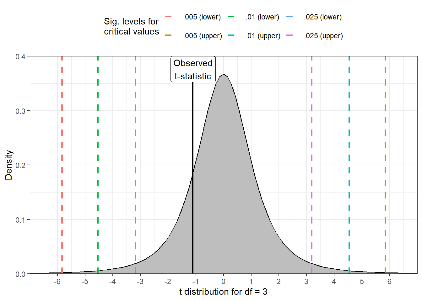
Which then leads us to \(t = \frac{-2}{1.78} = -1.12\).
To determine whether the result is statistically significant, we have to compare the obtained t-statistic to a t-distribution with 3 degrees of freedom (df). You can find the relevant critical values associated with a particular significance level for t-distributions of various degrees of freedom on page 543 of the Argyrous textbook.
Note 5.2: Degrees of freedom
The degrees of freedom of a dataset refers to the number of independent values that are free to vary without affecting the outcome of a calculation. In the above example, where we are interested in the mean of four datapoints, the degrees of freedom is 3. The first three values of the data can assume any value, but the fourth necessarily leads us to the sample mean. For one-sample t-tests (which also includes t-tests of regression slope coefficients), the degrees of freedom are always given by \(df = n - 1\).
We need to compare our observed t-statistic to the critical t-value associated with the conventional threshold for statistical significance (\(\alpha\)), which is .05. As we specified a non-directional alternative hypothesis, we look under the column “level of significance for two-tailed test”, allowing us to look for differences greater than or less than the value specified in the null hypothesis (in this case, 0). The relevant critical value for a t-distribution with 3 degrees of freedom is 3.182, meaning that we would expect to see a t-statistic at least as large as this five percent of the time over the long run, assuming that the null hypothesis is true. The t-value we calculated, however, is smaller than this value, meaning that its associated p-value is greater than .05 (although note that you cannot obtain the exact p-value associated with your test from the tables in the book). We should therefore NOT reject \(H_0\) and instead conclude that, in the population, the mean number of beers consumed by UvA students per week does not differ from 10. Formatting this in APA style, we have:
Our 1-sample t-test indicated that, in the population of Amsterdam students, the mean beers consumed per week (M = 8, SD = 3.56) did not differ from 10, t (3) = -1.12, p > .05.
5.2.1 Effect size: Cohen’s \(d\)
In the last lecture, you also learned about measures of effect size which can give us some information about the practical as opposed to statistical significance of our findings. These measures typically standardize effects such that they can be compared across different studies. To accompany t-tests, researchers typically use Cohen’s \(d\), which - in the one sample case - is computed as follows:
\[
d = \frac{\bar{x} - \mu}{s}
\]
As you can see, this resembles a signal-to-noise ratio which expresses differences in standard deviation units, allowing cross-study comparisons. For the data above, we compute as follows:
\[
d = \frac{8-10}{3.56} = -.56
\]
Like Pearson’s \(r\), there is a common heuristic for evaluating the absolute size of Cohen’s \(d\):
- \(d \le .2\) = small
- \(.2 < d \le .8\) = medium/moderate
- \(d > 8\) = large/strong
Thus, we could categorize the above as a moderate difference/effect.
Note 5.3: Statistical significance
To say that a finding is statistically significant does not mean that it is important; it merely means that the p-value produced by a null-hypothesis test falls below a specified \(\alpha\) level (usually .05) which gives the expected type-1 error rate of a test, in the long run. In other words, with \(\alpha = .05\) you expect your test to lead you to falsely reject \(H_0\) 1 in 20 times/5% of the time (i.e., to reject \(H_0\) when \(H_0\) is actually true), where p values \(< \alpha\) are typically accepted as sufficient for allowing one to reject \(H_0\). In the above example, the p-value associated with the t-test suggests that, assuming that \(H_0\) is true, we would expect to see a result at least as extreme as that which we observed 34.43% of the time, which is (naturally) greater than the 5% threshold, leading us to say that we fail to reject \(H_0\). If setting \(\alpha = .05\) seems arbitrary, that’s because it is - you will hear more about this towards the end of the course.
5.3 Confidence Intervals by hand
For our next trick, let’s imagine we sampled 100 UvA students and asked them to estimate how many shots of tequila they drink per weekend. We note a sample mean (\(\bar{x}\)) of 2.5, with a sample standard deviation (\(s\)) of 1.5 and we want to use these to estimate \(\mu_{tequila}\) in the UvA student population by building 95% confidence intervals, which will provide a range of plausible values.
Note 5.4: Confidence
The confidence level relates to the long-term coverage of the confidence intervals we generate. If we set the confidence level to 95%, then we expect that 95/100 confidence intervals constructed in this way over time should contain \(\mu\); however, that also means that 5/100 constructed intervals will NOT contain \(\mu\), and we cannot know whether the confidence interval we are currently building belongs to the former or the latter!
To construct the interval, we first need to calculate \(se\):
\[
se = \frac{1.5}{\sqrt{100}} = .15
\]
Next, to create the bounds of our 95% interval, we need to find the critical t-value which marks the top and bottom 2.5% of a t-distribution with \(df = 1 - n = 99\) degrees of freedom. Once more, we can find these from Argyrous, p. 543.
Now, we build the upper and lower bounds according to the following:
\[ ci_{95} = \bigg[\bar{x} - t_{crit} \times \frac{s}{\sqrt{n}}, \ \bar{x} + t_{crit} \times \frac{s}{\sqrt{n}} \bigg] \]
Plugging in the values gives us:
\[
ci_{95} = \bigg[2.5 - 1.98 \times .15,\ 2.5 + 1.98 \times .15 \bigg]
\]
\[
= \bigg[2.20 < \ 2.5 \ < 2.80\bigg]
\]
Given what we learned about confidence intervals above, we can conclude with something like:
With 95% confidence we estimate that the mean number of shots of tequila consumed per weekend in the population of Amsterdam students lies between 2.20 and 2.80.
5.4 One-sample t-test in SPSS
Let’s load in the ESS11 dataset and imagine that we are interested in working habits amongst men in Greece. Based on information from the Greek labour unions, we have reason to believe that Greek males normally work more than 40 hours per week on average, inclusive of overtime. This information is held in the variable wkhtot.
Before we go further, let’s formulate some hypotheses.
- \(H_0: \mu_{hrs} = 40\) (In the population of Greek males, average weekly working hours are not different from 40)
- \(H_1: \mu_{hrs} > 40\) (In the population of Greek males, average weekly working hours are greater than 40)
Note that we now have a directional alternative hypothesis (see Note 5.1). In this case, it can be justifiable to use a one-tailed t-test, meaning we only consider half of the t-distribution when deriving our p-value.
5.4.1 SPSS explainer video (ESS11)
- One-sample t-test (ESS11)
See video ‘ISA5’ here
5.4.2 Conclusion
In the population of Greek males, the total hours worked per week (inclusive of overtime) is greater than 40 (mean = 45.90, s = 13.36; t[1119] = 14.77, p < .001; Cohen’s \(d\) = .44).