4 Working with normal distributions II - the sampling distribution of means
4.1 Learning goals
4.1.1 Conceptual
- Understand the difference between a given variable’s distribution and the sampling distribution of means for that variable
- Answer questions about proportions/probabilities based on both types of distribution using z-formulae
4.1.2 SPSS
- Create new variables from existing values with
Compute
4.2 Recap: Z-transformations
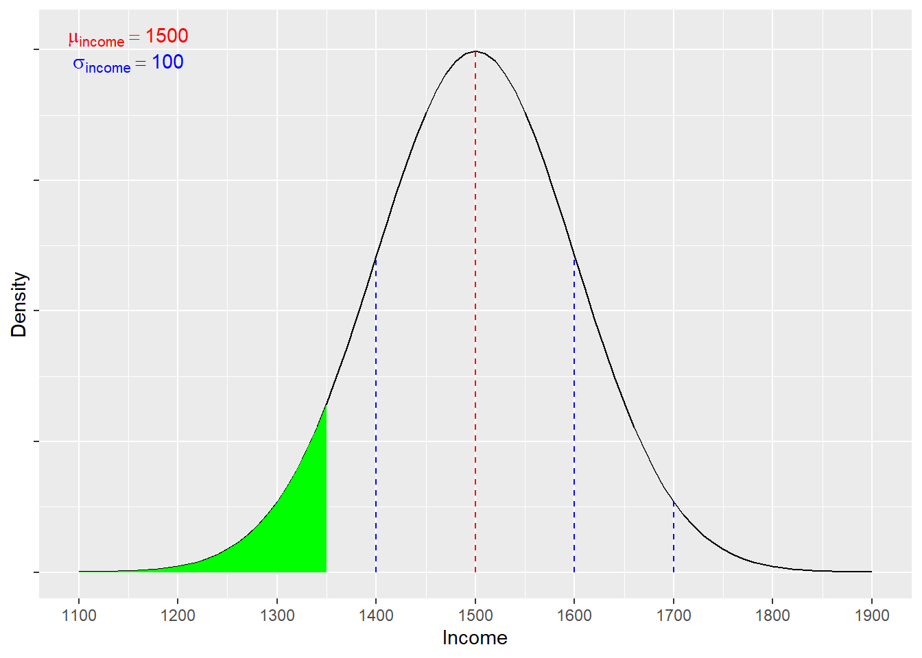
Imagine we know that income per week (in euro) is normally distributed in the population of Dutch university students who graduated in the last year, such that the mean (\(\mu\)) income is 1,500 EUR, with an SD (\(\sigma\)) of 100.We might wonder: what proportion of the population of new Dutch graduates would have a weekly income of less than 1,350 EUR?
We can see the area of interest in the distribution above, in Figure 4.1. To calculate the proportion, we first need to convert the target value into a z-score, which transforms the value into standard deviation units. In this case:
\[
z = \frac{x-\mu}{\sigma} = \frac{1350-1500}{100} = -1.5
\]
To work out the probability associated with a z-score of 1.5, we can consult the normal distribution tables in the Argyrous textbook (pp. 541 - 542), looking for the area under the curve beyond one point. This allows us to answer our question: there is a 6.68% chance of randomly selecting an individual with an income below 1,350 EUR per week from the population of new Dutch graduates
4.3 The Sampling Distribution (of Means)
Imagine (as before) that we know that income per week (in euro) is normally distributed in the population of Dutch university students who graduated in the last year (\(\mu_{income}= 1,500\), \(\sigma_{income}= 100\)). If we repeatedly draw samples of \(n\) = 1,000 from the population, then we might see \(\bar{x}_1=1,501.93\) , \(\bar{x}_2=1,497.62\) ,… and so on. Computing sample means from all possible samples of size \(n\) = 1,000 gives the sampling distribution of means (for \(n\) = 1,000).
The mean of the sampling distribution = \(\mu = 1,500\) and the standard deviation of sampling distribution is known as the Standard Error (SE). While the sampling distribution is purely theoretical (because we usually cannot collect all possible permutations of elements from our population), we can estimate the standard error of the sampling distribution of means with the formula:
\[
\sigma_{\bar{x}} = \frac{\sigma}{\sqrt{n}}
\]
Plugging in the values from our current example gives:
\[
\sigma_{\bar{x}} = \frac{100}{\sqrt{1000}} = 3.16
\]
We can now ask the question: what is the probability of drawing a sample (n = 1,000) from this population with a mean of less than 1,489 EUR?
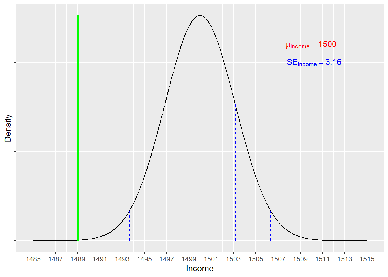
We can follow exactly the same steps as we did when working above with (fictional) population values:
\[ z = \frac{x-\mu}{\frac{\sigma}{\sqrt{n}}} = \frac{1489-1500}{3.16} = -3.48 \]
Our answer, then, is: there is a 0.02% chance of randomly drawing a sample (n = 1,000) with a mean income of less than 1,489 EUR from this population (with \(\mu = 1,500\) & \(\sigma = 100\))
4.4 SPSS explainer video (ESS11)
- Compute new variable from existing variables
See video ‘ISA4’ here